Can AI models work better together? Part 2: The missing baseline

In Part 1, Can AI models work better together? Part 1: Understanding road videos, I tested whether YOLO detections could help vision-language models (VLMs) count road users. The results looked mixed: adding YOLO reduced absolute count error for every tested VLM, but often lowered the graded score.

The measurements were correct for that setup. What I got wrong was treating a result from one weak detector as the broader fusion story.

Most of the experiment had focused on swapping VLMs while keeping the detector fixed. Once stronger YOLO models entered the comparison, the conclusion changed—and a baseline that had been sitting in the results all along became much more important.

Quick summary

• Increasing the nano detector’s input size helped, but moving from the nano model to the small model changed detected-count coverage about three times as much on this clip.
• With the stronger detectors, the YOLO-assisted pipeline beat the VLM-only pipeline for all five tested model tags. The graded-score gain ranged from 0.078 to 0.301.
• The comparison against YOLO alone told a different story. At the small and large detector settings, the mean fusion score fell slightly below the detector-only score. This was not universal: three tags still finished above the detector and two fell below it at each setting.
• A full-resolution check found genuine cars missing from the hand labels. That makes the top end of the comparison uncertain until all 26 frames are audited again.
• The most useful lesson is methodological: a system that combines a specialist with a general model should be compared against both components, not only against the general model.

This is still a 26-frame pilot from one counting clip. Each configuration was run once, and the fusion prompt contains an important confound discussed below. The crossover is a result to investigate, not a universal threshold.

The overlooked baseline

The counting experiment has four configurations:

Config	What it is
C0	YOLO only—return the counts directly from its detections
C1	YOLO detections passed to a text LLM, without the image
C2	VLM only—the image, without detections
C3	VLM + YOLO—the image, detections, and instructions for using them

Part 1 focused on C3 versus C2: does adding a detector improve the VLM pipeline? C0 was treated mostly as a reference point.

There is an equally important mirror question: does adding a VLM improve the detector? That is C3 versus C0. If the combined system costs more but cannot beat the specialist by itself, that matters—especially on an edge device with limited memory.

One detail is important throughout this article: C2 and C3 saw the same image, but C3 also received both detections and a dedicated instruction for using them. These are comparisons between two complete pipeline configurations. They do not isolate the causal effect of the detections alone.

Setup for this follow-up

This follow-up reuses the same 3840 × 2160 fixed-camera clip and the same 26 frames from Part 1. The hand labels contain 305 cars across those frames, plus a truck on 24 frames.

Five Ollama tags were tested: qwen3-vl:4b-instruct, gemma4:e2b, gemma4:e4b, minicpm-v4.6, and openbmb/minicpm-v4.6. The last two are tags from the same model family, so the equally weighted five-tag mean is not a five-family average.

For the new C3 runs, the VLM input width remained at 1920 pixels, the fusion prompt stayed at the same version, and only the detector changed. YOLO used a confidence threshold of conf=0.25. Each pairing was run once over the 26 frames.

The graded score ranges from 0 to 1, with higher being better. It gives partial credit based on relative count error for each road-user class present in a frame, with a penalty for hallucinated classes. Mean absolute error (MAE) shows how many objects the answer missed by. The fusion MAE comparisons cover the 50 present-class observations: 26 car counts and 24 truck counts.

The original detector baseline

Everything in Part 1 used yolo26n, the nano detector, at an input size of 1920 pixels. I selected it early, documented the reasoning, and then left the setting unchanged.

On the counting clip, that detector produced:

• 192 car detections against 305 hand-labeled cars, or 63% detected-count coverage;
• a truck detection on 6 of the 24 frames with a labeled truck; and
• a car undercount on all 26 frames.

The first measurement is detected-count coverage, not recall. It compares aggregate detection counts with aggregate hand labels; prediction boxes were not matched to labeled boxes at an intersection-over-union threshold. The fact that this ratio can exceed 100% later in the experiment is another reason not to call it recall.

The original C3 results therefore answered a narrower question than expected: does a detector that undercounts cars on every sampled frame help a VLM count? That is useful, but it is not the same as asking how fusion behaves as detector quality changes.

Climbing the detector ladder

The first step raised the nano detector’s input size from 1920 to 2560 pixels. The next steps kept 2560 fixed and moved to the small and large YOLO26 models.

Detector	Parameters	Weights	Cars detected / 305 labels	Detected-count coverage	Car MAE per frame	Direction of car error
yolo26n at 1920	2.6 M	5.5 MB	192	63%	4.35	26 under
yolo26n at 2560	2.6 M	5.5 MB	211	69%	3.62	26 under
yolo26s at 2560	10.0 M	20.4 MB	265	87%	1.69	19 under, 5 exact, 2 over
yolo26l at 2560	26.3 M	53.2 MB	323	106%	1.00	4 under, 8 exact, 14 over

On this clip, moving nano from 1920 to 2560 added 6 percentage points of detected-count coverage. Moving from nano to small at the same 2560 input added another 18 points—about three times as much. The move to large added another 19 points.

The shape of the error changed too. Both nano configurations undercounted on every frame. The small and large detectors made errors in both directions and had lower car MAE against the existing labels.

What does 106% coverage mean?

The large detector found more cars than the hand labels said were present. That 106% ratio has at least two possible explanations: the detector produced false positives, or the human labels missed small cars. Both can be true at the same time.

Three observations suggested that missing labels were part of the problem:

1. Car MAE against the existing labels fell from 1.69 for the small model to 1.00 for the large model even as the total detection count rose.
2. The large model’s frame-level errors appeared on both sides of the labels: 14 over, 8 exact, and 4 under, with a range from −1 to +3.
3. Raising the confidence threshold to conf=0.4 reduced aggregate coverage to 98% but changed car MAE only slightly, from 1.00 to 0.96.

Those checks are suggestive, not proof. To look more closely, I inspected the worst apparent overcount. On frame 510, the large detector counted 13 cars while the hand labels said 10. Here is the far half of the 4K frame, enlarged:

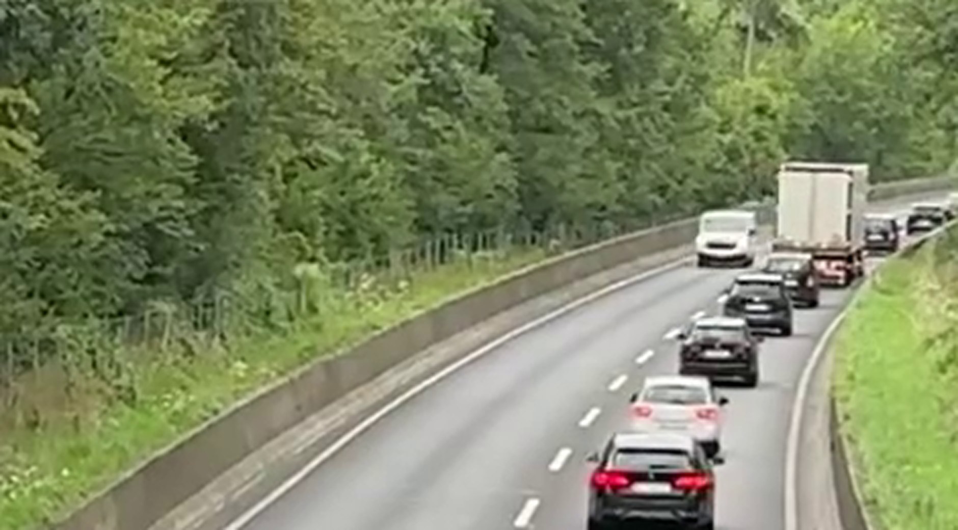
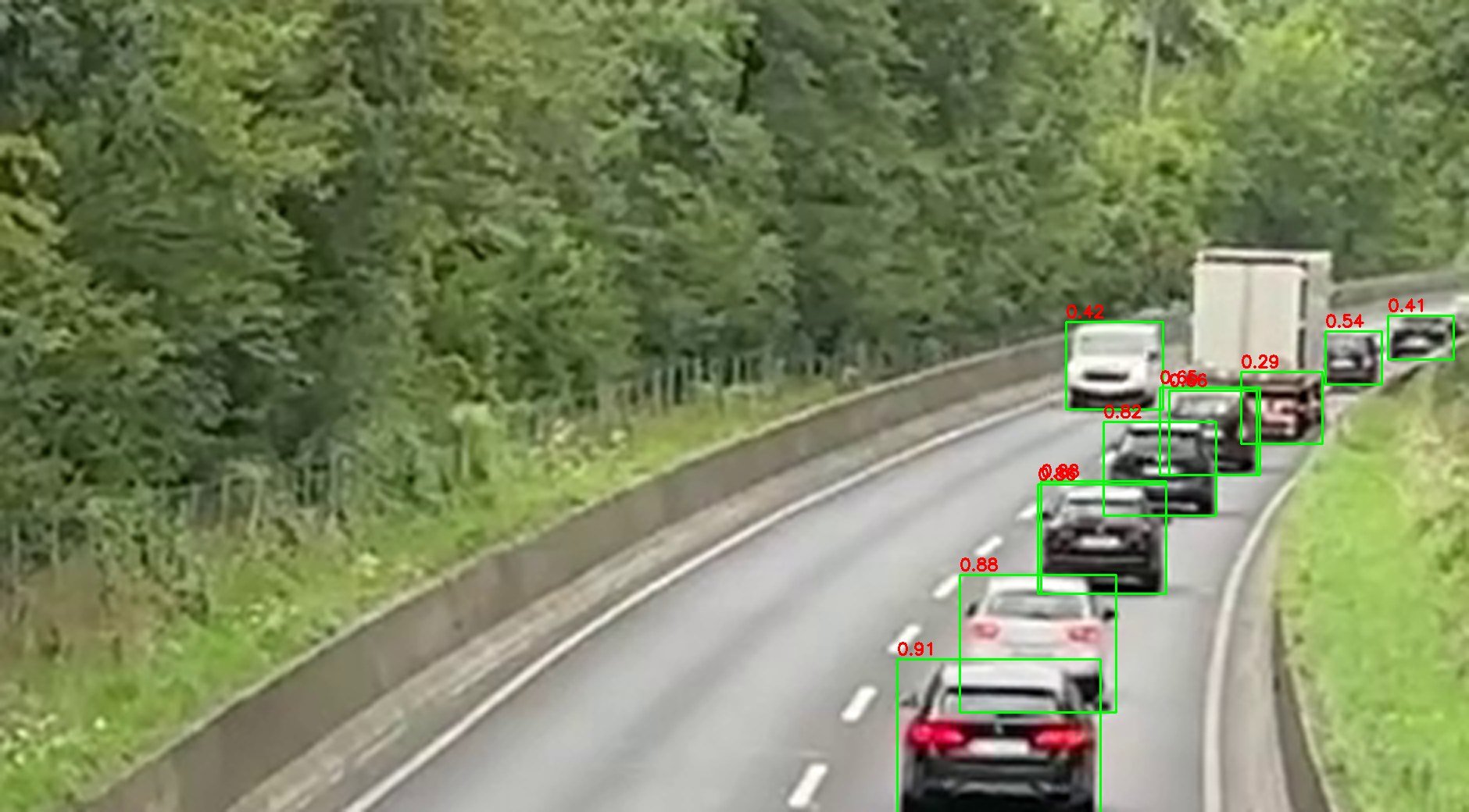
Several apparent surplus boxes sit on genuine far-field vehicles in the receding queue. They are easy to miss in the 1280-pixel review frames used for labeling.

This check confirms that at least some of the apparent surplus comes from missing labels. It does not show that every detection across all 26 frames is valid. Until the labeling is repeated at full resolution or every box is audited, the labels are not reliable enough to rank small differences among the top configurations confidently.

The average crosses over

The first comparison repeated the original C3-versus-C2 test: fusion versus the VLM-only pipeline. With yolo26s or yolo26l, all five tested tags beat their paired C2 score. The graded-score gains ranged from 0.078 to 0.301, while MAE fell by 1.26 to 2.40 objects per present-class observation.

That is much cleaner than the Part 1 result. Better detector input improved the complete fusion pipeline for every tested tag. Because C3 also had a different instruction, however, the whole change cannot be attributed to detections alone.

The second comparison put C3 against C0: does the combined pipeline beat returning YOLO’s counts directly?

Detector	C0 alone	Mean C3	Best C3	Mean C3 − C0
yolo26n at 1920	0.460	0.518	0.579	+0.058
yolo26n at 2560	0.567	0.627	0.665	+0.060
yolo26s at 2560	0.791	0.768	0.810	−0.023
yolo26l at 2560	0.798	0.767	0.837	−0.031

The mean changes sign. With either nano detector, the average C3 pipeline beats the detector alone by about 0.06. With the small and large detectors, the average falls slightly below C0.

This is not a universal per-model crossover. At both stronger-detector settings, three tags remain above C0 and two fall below it. For yolo26l, the positive margins range from about 0.001 to 0.038. The low gemma4:e4b result—0.623 against C0’s 0.798—pulls the mean down substantially.

So the honest summary has two parts:

Fusion beat the VLM-only pipeline for every tested tag, but the average fusion pipeline did not beat a strong detector on its own.

Both statements come from the same runs. The first says that better specialist input helps the general model pipeline. The second says that adding a general model is not automatically useful once the specialist is already strong. Whether the extra VLM is worthwhile depends on the model tag, the task, and the cost—not only on the mean.

Why the second baseline matters beyond YOLO

When a specialist and a general model are combined, there are two natural baselines:

1. the general model without the specialist; and
2. the specialist without the general model.

Comparing only with the first baseline answers whether specialist input helps the general model. It does not answer whether the combined system is better than its simpler component.

The error pattern suggests a working hypothesis for the next experiment. A detector that was always low gave the lower-bound fusion prompt a simple correction to encourage: look for missed objects and revise upward. Once the detector’s errors appeared in both directions, there was no equally simple adjustment. That could explain why some VLM tags stopped adding value—but the current prompt prevents a causal conclusion.

The OCR experiment from Part 1 hinted at a related pattern. OCR helped dramatically when it found a place-name clue that the VLM had missed, but was neutral or harmful when the VLM had already read the important sign. That was a separate two-clip pilot with changing OCR settings, not an independent replication of this crossover. It does reinforce an important question for every combined system: what unique information does each component contribute?

For a retrieval pipeline, a tool-using agent, or OCR paired with a model, the inexpensive check is the same: score each meaningful component on its own and put those results beside the combined system.

What this changes for the edge-device plan

The target for this project is still an 8 GB Jetson Orin Nano. These PC results changed the next set of tests, but they do not establish what will fit or how fast it will run.

At 2560 pixels, moving from yolo26n to yolo26s added 7.4 million parameters and about 15 MB of weights. On this clip, the detector-only graded score rose from 0.567 to 0.791. In the cached two-stage experiment, YOLO runs once before the VLM tests, so its latency is outside the measured VLM path. A live Jetson pipeline will need both components measured together.

The preferred VLM partner changed as the detector improved. With the original nano detector, qwen3-vl:4b-instruct gave the best fusion result. With the stronger detectors, a MiniCPM tag produced the best cell in the matrix: 0.837 graded with an MAE of 0.64.

The isolated Ollama measurements on the PC were about 7.4 GiB resident for qwen3-vl:4b-instruct and 1.0 GiB for minicpm-v4.6; their downloads were different from runtime memory. These are useful screening measurements, not proof of Jetson fit. The next step is to benchmark the selected detector and VLM together on the actual device, including memory, latency, and power.

The practical lesson for now is that the edge VLM should not be chosen before fixing the specialist configuration. The ranking applies to a pair, not a model in isolation.

What could change this result

Four limitations matter most.

1. The prompt no longer matches the detector. The fusion prompt calls detections a lower bound and warns that the detector misses small or distant objects. That was broadly accurate for the nano detector, which undercounted cars on every frame. It is not accurate for yolo26l, which overcounted against the existing labels on 14 of 26 frames. A symmetric prompt could change the C3 results substantially.
2. This is one relatively easy clip. The counting clip uses a fixed camera on flowing traffic, with large scale variation but little occlusion. A crowded junction, night scene, or unfamiliar class could produce a different pattern.
3. The labels need a full-resolution audit. Frame 510 proves that the current labels omit some visible cars. Until all 26 frames are relabeled or audited, the top-end differences remain uncertain.
4. The sample is small and not fully independent. This is one run per configuration, four detector settings, and five VLM tags. Two tags come from the MiniCPM family. Replicated runs, more model families, and more clips are needed before estimating where—or whether—the mean crossover repeats.

None of those limitations changes the methodological lesson: a combined system should be reported beside both single-system baselines. The detector-only baseline was present in every run but did not receive the attention it deserved.

That is the result going into the Jetson stage: improve the specialist first, then make every other component earn its memory and inference cost.